Seriesly Internals Tour
My previous a blog post introduces a documented-oriented time series database I wrote. It’s introductory material that somewhat describes why the software exists and a bit about how to use it.
Here I describe how it works. As mentioned before, the bulk of the software was in a useful state in two weeks. I attribute much of this success to go. The code itself contains the details of my knowledge, but I’ll highlight some of the parts that helped the most in the coming paragraphs.
The process described in the following paragraphs generally occurs in under a millisecond, in my installations. On a sufficiently large, cold query, it could theoretically take several minutes.
Logical Overview

The query model is as simple as I could meet all of my current use cases with.
The diagram to the right represents a logical overview of a query flowing through the system.
Understanding the Query
First, the HTTP query is parsed and put into a struct that represents
the information that’s needed. Here we validate and parse the from
and to timestamps, the grouping, the reducers, etc…
Also, we place a before timestamp that is the latest possible time
for us to do any work on this query (queries that would run longer
than the server’s configured max query time are aborted even if
partially processed).
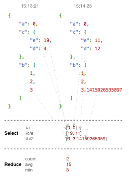
Most importantly, there’s some output data in the struct. The following example should aid in understanding. Start with an input query:
/testdb/_query?from=1347469924&to=2013&group=3600000&ptr=/a&reducer=min
That will map to a queryIn struct that looks like this:
queryIn{
        dbname: "testdb",
        from: time.Date(2012, 9, 12, 10, 12, 4, 0, time.UTC},
        to: time.Date{2013, 1, 1, 0, 0, 0, 0, time.UTC},
        group: 3600000,
        ptrs: []string{"/a"},
        reds: []string{"min"},

        // Control, logging, timeout, etc...
        start: time.Now(),
        before: time.Now().Add(queryTimeout),
        started: 0,

        // Output channels
        out: make(chan *processOut),
        cherr: make(chan error),
}
The started int is a counter that’s incremented (atomically) each
time a grouping is located. All of the final responses are fed into
the out channel. Once the query worker completes walking the tree,
it will send its return value (generally nil) into cherr,
informing the HTTP handler that all groupings have been found and
started will no longer increase.
Locating the Relevant Documents
The query processor server is asynchronously walking the docs to locate the ones that apply to the query. Once the query is submitted, the HTTP handler no longer pays any attention to the query directly.
But the actual query processing is where we start needing to tighten resource controls. In theory, we don’t need more queries digging through storage than we have the resources to process. In practice (it’s all configurable), oversubscribing doesn’t seem to make anything faster, but leads to a lot of memory bloat as more things are stuck in progress.
Without delving too deeply into queueing theory, let’s just imagine you’re at a well-organized bank where you’ve got a single line and four identical tellers.

The number of workers is fixed throughout the lifetime of a process and each has one simple job:
to transform a query to a collection of grouped document IDs to be handled by a doc processor on behalf of a client
That’s it. One of the workers takes the request off the queue, starts
digging through documents between the from and to range of the
query emitting a batch when it crosses every boundary defined by
group and passes it down to a doc processor.
It’s important to note that both the queues into and out of the query processor are blocking, at least, eventually. By default, an HTTP client will block on submitting his query until a worker is available and a query worker will block on submitting a batch to doc workers until a doc worker is available. Both of these things are configurable, but in practice, letting work build up between these areas increases memory overhead without getting more work done sooner.
Processing Documents
The document processors are another group of identical workers with another fairly simple job:
to read a collection of documents, extract relevant information from them, and reduce the extracted information to an output value
Extracting a portion of the query example document from the intro blog post, you can see the role it performs to the right.
Before it begins pulling documents, it creates one goroutine for each reduction that was requested for the result. I’ll describe this pattern more below, but at this point it’s important to understand that we’re going to be streaming data through the reducers and not accumulating and batch processing results.
The most expensive things it does are also least interesting, so I’m
going to be a bit hand-wavy. It fetches the document from disk (which
is pretty much pread) and parses it as a json document.
Ignoring all the gory details of coercion, error handling, etc… that gives us a loop that looks like this:
// Build the slice of reducers
reducers, outputs := makeReducers(reds)
// Pull each document from storage
for _, data := range docs {
    jsondoc := parseJson(data)
    for i, jsonpointer := range ptrs {
        reducers[i] <- extractValue(jsondoc, jsonpointer)
    }
}
// Close reducer input channels so they complete
closeAll(chans)
// Read the output of the channels and send it all back
results <- recvItemFromAllChannels(chans)
Due to the way this is streamed, we never require more than one document in memory per document worker. A typical reducer for gauge values doesn’t need more than its return value resident.
Closing the reducer input channels causes them to emit their results on an output channel. Harvesting all these results for a “row” joins all the goroutines and allows us to emit the value back to the HTTP worker so it can transmit the results (described in further detail below).
“But wait,” you say, “what are these goroutines that are being joined?”
Every column in every row is a goroutine. e.g. a 2,000 row result with 100 pointers and reducers applied requires at least 200,000 short-lived goroutines to be started to model this concurrency.
Now, I imagine many of you are wondering why I’d make reducers be functions that are run in separate goroutines that keep their state on the stack and then consume a channel of input. Why wouldn’t I just make them structs where their state is held as a field and then just have a method called on the input to modify the state?
Because that’s hard. Consider the c_min reducer to understand why:
func(input chan ptrval) interface{} {
    rv := math.NaN()
    for v := range convertTofloat64Rate(input) {
        if v < rv || math.IsNaN(rv) {
            rv = v
        }
    }
    return rv
}
The c_min reducer computes the minimum growth rate (per second) of a
stream of pointer values on the given channel. The trick is that in
order to know the rate at a given instance, I need to know both the
next value and the timestamp of the next value so I can divide the
growth rate over the time delta.
It’s all obvious once you consider how convertTofloat64Rate must
work. This is a function that takes a stream of ptrvals and emits a
string of float64s that are flattened rates over that range. It
does all of the hard work around finding the first suitable value
(skipping nil values where the pointer didn’t point to valid data)
and computing the delta from each previous value to emit. By
definition, this always consumes more values than it emits.
Perhaps my brain is twisted by decades of living in unix shells, but I do the same thing processing data in the shell:
% grep field fromfile | ./computerate | ./min
Except goroutines are way cheaper than threads (which are way cheaper than processes), so the way that’s natural to me also performs quite well. This is certainly possible to do with OO-style state management, but I don’t want to write that code.
As a bonus, convertTofloat64Rate (and its older brother
convertTofloat64) creates a goroutine that consumes the input
channel in order to emit over its output channel. That means that if
all 200,000 of the results were numeric, it’d require 400,000
goroutines.
Transmitting Results
Meanwhile, back in the HTTP handler…
After it submitted the request, the HTTP handler started a select
loop across the two channels built at query time. We’ll call them the
error channel and results channel.
When the error channel has received its completion message and there has been one grouping output for every grouping found by the walker (the counter mentioned above), the query processing is complete.
The HTTP layer currently emits docs as soon as they come out of the results channel, this brings two great benefits:
The first result latency is as low as possible. Once a result is known, we immediately transmit it. Early versions batched up the results and would get similar throughput, but I decided it was unnecessary.
Memory usage is as low as possible. Since I’m not batching up the results (and more importantly, not serializing them into a in a single encoder call), memory usage is down to the minimum required to pass the necessary information around and encode it for the wire.
However, these benefits come with two consequences:
Groupings are not returned to the HTTP requester in any defined order. In fact, if you run the same query twice, you will get the same results, but with different time windows appearing in different locations in the result. This is especially strange if you stream compressed data from the server and see it coming back as different sizes with the same canonical document representation.
There’s no clean way to report an error in an HTTP stream. After I
send HTTP 200 and start streaming data, it’s too late to realize
there’s a problem and call it a 500. The best I can do is hang up
and leave you with an invalid document.
I struggled with this one a bit, but not having to buffer into memory, reducing latency, etc… while not having a great answer for large broken queries seemed like a good trade-off. Most ways I could figure to send someone an error in-stream in the rare case where one happens would complicate the user experience. With this approach, even completely cold queries return results pretty much immediately.
About Storage
Seriesly uses couchstore for the backend. Depending on how intimately you know CouchDB, you can think of it as a C implementation of the core storage of CouchDB. Except, of course, I’m using my go bindings.
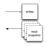
Couchstore provides an on-disk append-only b-tree. This gives me a durable format I can write to and read from at the same time. Neither readers nor writers pay any attention to each other whatsoever. Each query or doc worker opens a database for read access whenever it’s necessary and just starts reading. If a write is happening at the time, the reader just seeks backwards a bit in the file until it finds a valid previous header and carry on.
Writes are batched by time and/or size. That is, a write targeting a database doesn’t immediately hit the filesytem. This is mostly beneficial when loading lots of data in bulk. Obviously both of these parameters are configurable.
If most of the writes are small, you’ll want to compact the database periodically. Compaction never blocks reads and almost never blocks writes. There’s a buffered channel between the HTTP handler for storing a new document and the actual DB writes. If you exceed this buffer size, the put will block. Otherwise, writes are flushed, compaction occurs, the DB is atomically replaced and then the accumulated writes are completed.
Now with Memcached
The above all assumes no cache. Throwing memcached in the mix makes things a lot more interesting. Let’s take the first diagram and fit a cache into it:
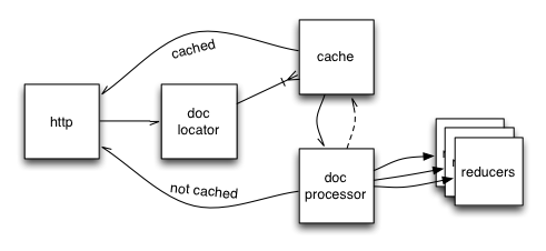
Now, conceptually, the cache just interposes between the query workers and the document workers. The code is very close to that, in fact. If you don’t have memcached enabled, the channel that the query worker places its requests into is the document worker input itself. When you have memcached enabled, the query worker output goes to the cache workers (and cache misses go to the document workers).
What’s unusual about the cache usage here is that I’m not using any patterns I’ve used elsewhere with memcached. It’s a little similar to how the internals of spymemcached were implemented, but I did some interesting binary-protocol-only stuff.
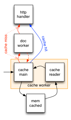
The diagram to the right shows the approximate anatomy of the
memcached workers and their interaction with the rest of the system.
The orange box delineates the conceptual memcached worker from the
rest of the system. Note that a memcached worker is two goroutines
sharing a connection to memcached. One only reads and one only
writes. I labeled the one that writes as main as it’s also our
interface to the cache.
Unlike most uses of memcached, we don’t do any “multi” type operations
like a “quiet” get at all. Instead, any time we need to send data
to memcached, we construct a packet and lob it over. The reader is
reading the output of that and after parsing the result into a packet
and determining that the main goroutine might be interested in it
(basically, this means it’s a successful get request), it sends it
back. These two messages are stitched together using the memcached
binary protocol opaque field – a 32-bit number that is application
specific and designed to enable this type of thing.
Pseudocode of our memcached main looks like the following:
for {
    select {
        case req := <-cacheRequestChannel:
            // Generate a unique identifier for this request
            opaque := nextOpaque()
            opaqueMap[opaque] = req
            mc.transmitGetRequest(req.key, opaque)
        case res := <-cacheResponseChannel:
            // Map the response back to the request by identifier
            in := opaqueMap[res.Opaque]
            delete(opaqueMap, res.Opaque)
            if in.err {
                docProcessor <- in
            } else {
                in.response <- res
            }
        case toSet := <-setRequestChannel:
            mc.transmitQuietSetRequest(toSet.key, toSet.value)
    }
}
Where a typical “multiget” type strategy would require you to batch up a bunch of requests, send them all, get all the responses and infer the misses, we process the results with minimal state – only keeping up with what we’ve got in-flight. If a response is a hit, we send it back up to the http handler. If it’s a miss (or there was any other error), we send it to the doc worker. Done.
Of course, the actual loop is a bit more complicated as it deals with fetch cancellations, connection failures which result in dumping all in-flight cache requests directly into the document worker queues while asynchronously starting a timed reconnection loop and a few other things. The above is pretty much the golden path, though.
At the layer the cache is installed, there are a lot of benefits I don’t get, but when the site was pretty popular on hacker news, I was seeing queries like this flying by:
Completed query processing in 69.528ms, 9,394 keys, 1,920 chunks
That means we pulled 9,394 document IDs from the on-disk index,
chopped them up into 1,920 groups, computed hash keys for them and
then passed through the above select loop 3,840 times (once each for
1,920 requests and again for the responses) in 69.528 milliseconds.
Under load. That’s an absolute ceiling of 35µs cache round trip time,
again, ignoring all other queries running at this time.


