conc Lists in Erlang - Or Making the Kessel Run in 12 Parsecs

I saw this wonderful Guy Steele talk titled Organizing Functional Code for Parallel Execution.

The talk describes how what we have learned to get us this far may be preventing us from proceeding in the new world of many cores.

I don’t want to ruin the whole talk for you, you should watch it and learn great things, but I found one thing quite inspirational. In his description of behaviors of conc lists (which I’ll go into more below), he described the time complexity of doing a mapreduce of his conc list as logarithmic.

This blew my mind. mapreduce n items in O(log n) time. I was fascinated. I could read the code, but I had to touch it, so I built an implementation of conc lists in erlang to try it out.

Quick Intro to cons Lists

conc lists are described in contrast to cons lists, so I’ll do a quick review on those first.

A cons list is basically a pair. In lisp, the first element is called a car and the second element is called a cdr, but we’re talking about erlang here where you typically just pattern match stuff, so I’ll just write the lists out in erlang notation and rip them apart with pattern matching.

The empty list is represented as []. It’s boring, but note that it’s at the end of every list. So if you see a list that looks like it has one element: [a], the cons cell is really the pair of a and [].

In erlang, cons looks like this: [SomeElement | RemainingList]. You can cons the single element above as [a | []]. A three element list can be expressed as [a, b, c] but you can also think of the implementation as [a | [b | [c | []]]].

This is significant when it comes to implementing code to process cons lists, because this is how you can model traversal operations such as map, foldl, length, etc… in your head. Each splits the list into the first element and the rest of the elements, performs an operation on the first element and then recurses over the rest.

Length, for example, may be implemented as follows:

length([]) -> 0;                   % Empty list is terminal.
length([Hd|Tl]) -> 1 + length(Tl)  % Recurse on elements.

Now for the good parts…

Quick Intro to conc Lists

conc lists point in two directions instead of just one. They’re really more like trees. Of course, there’s nothing stopping an implementation from having further dimensions, but that’s an exercise for the one doing the profiling.

Unlike a cons where you really only have two things (an element or the empty list), in a conc, you have three:

null is analogous to its cons empty cell. It is the end of the road and contains no data and no pointers elsewhere.

A singleton contains exactly one element and nothing else.

A concatenation contains a left and a right pointer which each may be to another concatenation, a singleton, or null.

Unlike a typical binary tree structure, these have no natural ordering, so at this point, we consider every operation to be O(n). In a moment, we will begin violating this, but in the meantime, let’s draw some pictures.

There are many ways to represent the same conc list. The original presentation went over a bunch, but I’ll just illustrate two here.

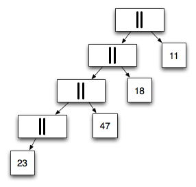
We’ll use [23, 47, 18, 11] for the purpose of example, because he did and he’s awesome.

To the right, we see what an unbalanced conc list representation of our list might look like.

If you are familiar with trees, you can see that an in-order traversal will visit each element in the same order as our cons representation above.

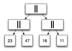
To our left, we see the same conc list in a well-balanced form.

And this is where things begin to get interesting.

conc List Processing

conc lists have two fundamental operations: append and mapreduce.

append(A, B) puts can be thought of as building a concatenation of A to B (though we do something a bit more optimal in implementation to avoid unnecessary concatenation cells).

mapreduce isn’t quite the same thing as a lists:mapfoldl, so don’t let that confuse you. You can imagine a simple implementation of a cons mapreduce looking like this:

mapreduce(MapFun, ReduceFun, Initial, List) ->
    lists:foldl(ReduceFun, Initial,
                lists:map(MapFun, List)).

Of course, we don’t don’t do two passes through the list. In fact, assuming we can keep our conc lists balanced, we get to perform linear-complexity operations in logarithmic time.

First, let us consider a naive implementation of a conc mapreduce:

mapreduce(_Map, _Reduce, Id, null) ->
    Id;
mapreduce(Map, _Reduce, _Id, {singleton, I}) ->
    Map(I);
mapreduce(Map, Reduce, Id, {concatenation, A, B}) ->
    Reduce(mapreduce(Map, Reduce, Id, A),
           mapreduce(Map, Reduce, Id, B))

The length operation, for example, just maps each element to 1 and then reduces the sum of all mapped numbers. This includes the sum of the sums as it walks up the tree. Consider the code for length:

length(L) ->
    mapreduce(fun (_X) -> 1 end,
              fun(X,Y) -> X+Y end,
              0,
              L).

If you consider the balanaced list from above, the process of computing the length is to mapreduce the left path, then the right and then reduce the results of each, or (1 + 1) + (1 + 1).

Going Parallel

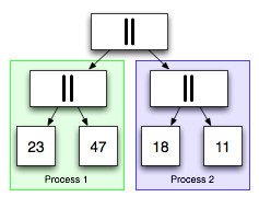
The secret is that a balanced conc list may be split in half in constant time.

In the mapreduce implementation, each concatenation is a point where we can parallelize the computations of the mapreduce to the left and the mapreduce to the right and then reduce them together as the computation completes.

So in a practical application, length will concurrently compute the left list’s (1 + 1) and the right list’s and (1 + 1) and then reduce them with the final summation of (2 + 2) after they finish.

On a small scale, this looks boring, but consider the following example:

C = conc:from_list(lists:seq(1, 1000)).
timer:tc(conc, mapreduce,
         [fun(_) -> timer:sleep(1000), 1000 end,
          fun(X, Acc) -> X + Acc end,
          0,
          C]).

Here, we take a 1,000 node conc list and perform a mapreduce on it where the mapping function artificially takes 1 second (1000ms) to complete, and then returns that same 1000 as the map result. The reducer then adds all of those milliseconds together.

I’m using the timer:tc function here to show the magic of auto-parallelization in the conc mapreduce. That unfortunately makes the invocation look a bit funny, but anyone who’s programmed in erlang has done plenty of similar M,F,A invocations, so I hope it’s not terribly confusing.

There result of that call is {4013058,1000000} – that is, 4,013,058µs to perform 1,000,000ms worth of work.

The units are kind of confusing – complain to the erlang guys about that. Convert them both to seconds and you’ll see that I did 1,000 seconds worth of work in 4 seconds (and you feel that when you do it interactively).

I Want to Play

I’ve got a repo up on github with my code. The mapreduce parallelism seems about right (though it’s not depth-limited), but rebalancing is suboptimal.

I look forward to your contributions to make this implementation better, but thanks go to Guy Steele for the linked list of the future.